Solving a PDE in complex geometries with the smoothed boundary method.

We have also included functionality for solving PDEs in arbitrary geometries using the smoothed boundary method. We demonstrate with the 2D Allen-Cahn equation in this example.

import jax.numpy as jnp
import numpy as np
from jax import random
import matplotlib.pyplot as plt
from IPython.display import HTML
import matplotlib.animation as animation
import diffrax as dfx
from PIL import Image
import numpy as np

from mosaix_pde.numerics.domains import Domain
from mosaix_pde.numerics.shapes import Shape
from mosaix_pde.numerics.equations.allen_cahn import AllenCahn2DSmoothedBoundary
from mosaix_pde.pde_model import PDEModel

We will solve the PDE on a smiley face with sunglasses.

# Load image and convert to grayscale
img = Image.open('../cool_smile.png').convert('L')

# Convert to numpy array and binarize
img_array = np.array(img)
binary = (img_array > 128).astype(np.float32)  # Threshold at 128

# Convert to jax array
binary_mask = jnp.array(binary)

We create a shape from the binary mask. This will run the smoothing algorithm to get a mask with a smooth boundary.

There are four important parameters in the smoothing process. The first is the smooth_epsilon, which controls the energy of the smoothing. A larger number will produce more smoothing. The second is the smooth_curvature. A value of 1 will reduce curvature in the shape. A value of zero will not change the shape’s curvature. Usually, a small number like 0.005 is good as it has little impact on the overall shape, but smooths out pixelated artifacts. The third is the smooth_dt. The smoothing process involves solving a modified time-dependent Allen-Cahn equation. This is the time step for solving the PDE. The fourth is the smooth_tf. This is how long the PDE is simulated forward in time. A larger value will produce more smoothing.

shape = Shape(
    binary=jnp.array(binary_mask),
    dx=(1.0, 1.0),
    smooth_epsilon=3.0,
    smooth_curvature=0.008,
    smooth_dt=0.01,
    smooth_tf=100.0,
)

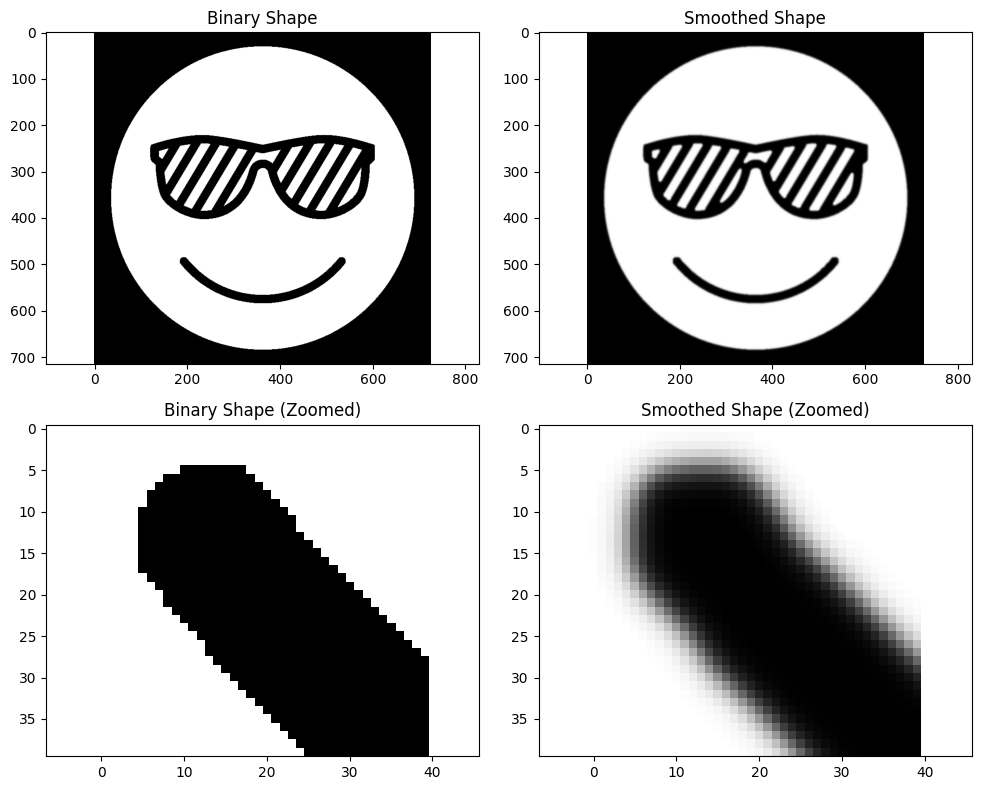
We can now visualize the results of smoothing the geometry.

fig, ((ax1, ax2), (ax3, ax4)) = plt.subplots(2, 2, figsize=(10, 8))

ax1.imshow(shape.binary, cmap='gray')
ax1.set_title('Binary Shape')
ax1.axis('equal')

ax2.imshow(shape.smooth, cmap='gray')
ax2.set_title('Smoothed Shape')
ax2.axis('equal')

ax3.imshow(shape.binary[480:520, 180:220], cmap='gray')
ax3.set_title('Binary Shape (Zoomed)')
ax3.axis('equal')

ax4.imshow(shape.smooth[480:520, 180:220], cmap='gray')
ax4.set_title('Smoothed Shape (Zoomed)')
ax4.axis('equal')

plt.tight_layout()
plt.show()

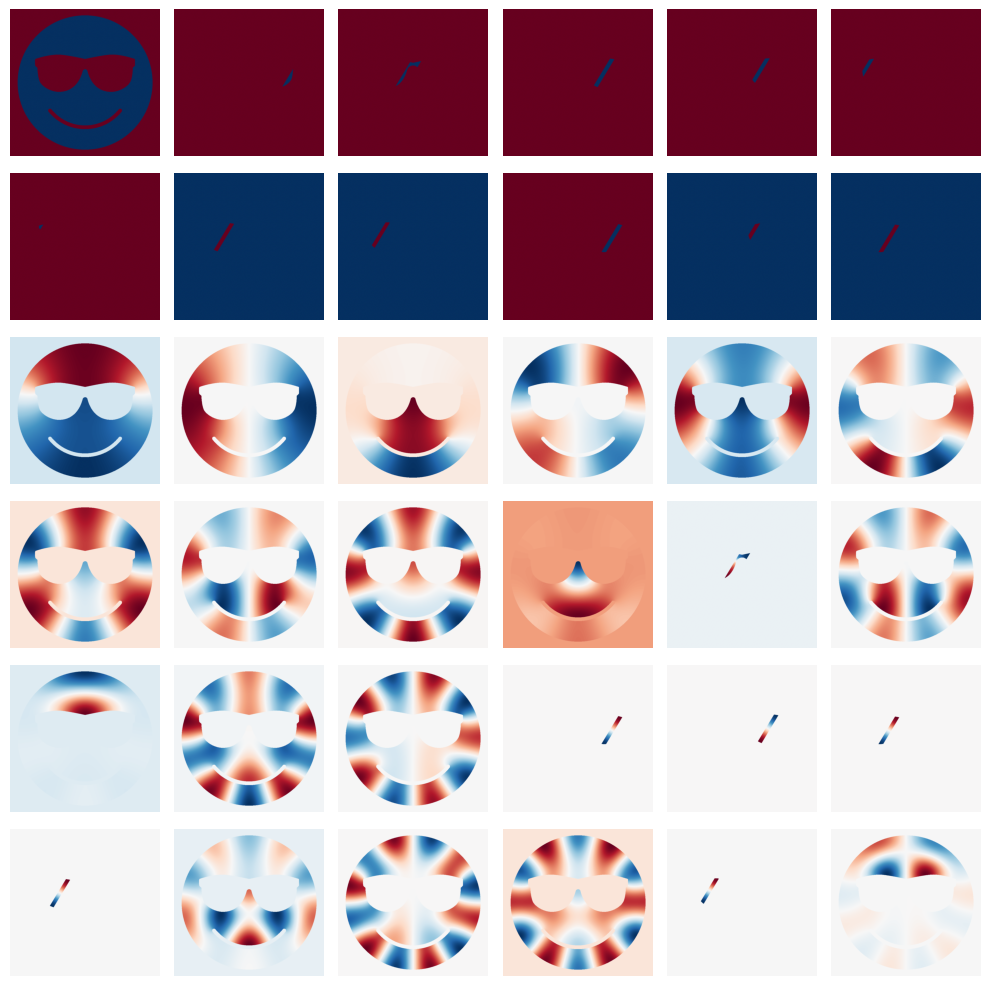
While not used in this example, we can also compute the eigenvectors of the graph Laplacian that make up the geometry. This is useful if performing some optimization where when parameter is a function on the domain. You can get an orthornormal basis for the domain using the eigenvectors of the graph Laplacian.

Here, we compute and visualize what these shape modes look like.

shape.get_shape_modes(N=36)

# Plot shape modes
fig, axes = plt.subplots(6, 6, figsize=(10, 10))
axes = axes.flatten()

for i in range(36):
    axes[i].imshow(shape.shape_basis[:, :, i], cmap="RdBu")
    axes[i].axis("off")

plt.tight_layout()
plt.show()

Nx, Ny = binary_mask.shape
Lx = 0.01 * Nx
Ly = 0.01 * Ny

domain = Domain(
    (Nx, Ny), ((-Lx / 2, Lx / 2), (-Ly / 2, Ly / 2)), "dimensionless", shape
)

model = PDEModel(AllenCahn2DSmoothedBoundary, domain, dfx.Tsit5)

t_start = 0.0
t_final = 20.0
dt = 0.000001
ts_save = jnp.linspace(t_start, t_final, 200)

pde_parameters = {
    "kappa": 0.002,
    "f": lambda c: c * jnp.log(c) + (1.0 - c) * jnp.log(1.0 - c) + 3.0 * c * (1.0 - c) + 0.059,
    "mu": lambda c: jnp.log(c / (1.0 - c)) + 3.0 * (1.0 - 2.0 * c),
    "R": lambda c: (1.0 - c) * c,
    "theta": lambda t: jnp.pi / 2.0,
    "derivs": "fd"
}

key = random.PRNGKey(0)
u0 = 0.5 * jnp.ones((Nx, Ny)) + 0.1 * random.normal(key, (Nx, Ny))

solution = model.solve(
    pde_parameters,
    u0,
    ts_save,
    stepsize_controller=dfx.PIDController(rtol=1e-4, atol=1e-6)
)

fig, ax = plt.subplots(figsize=(4,4))

ims = []
for i in range(0, len(solution), 10):
    im = ax.imshow(solution[i] * domain.geometry.binary, animated=True,
                   vmin=0.0, vmax=1.0,
                   extent=[domain.box[0][0], domain.box[0][1],
                          domain.box[1][0], domain.box[1][1]])
    ims.append([im])

ani = animation.ArtistAnimation(fig, ims, interval=200, blit=True)

plt.title('Allen-Cahn Evolution with Smoothed Boundary')
plt.xlabel('x')
plt.ylabel('y')

plt.close()

HTML(ani.to_jshtml())

Once Loop Reflect